How Can I Add a Cell Border to an Excel Spreadsheet Value?

With all the fancy 3D virtual world systems grabbing headlines, it’s reassuring to find someone who’s interested in information about one of the original applications of personal computers: spreadsheets. Indeed, it’s a program called Lotus-1-2-3 that really helped establish the value of computers for non-corporate users back in the darn of the PC era, with people marveling how they could balance their checking account on the computer. Definitely back in the day! For the vast majority of people back in that era, this was pre-Internet too, so they were using their hardwired phones stuck in acoustic gadgets to “talk” with another computer as a way to go online. The pinnacle of that era was the weekly AOL discs in the mail: logging in to America Online was the height of wired computing!

All these decades later and it turns out that spreadsheets are still darn useful for financial projections or even just to offer up the foundations of a visual presentation of numeric data. Want to “what if” your mortgage payments if the prime interest rate goes up or down a few percentage points? Easily done. Balance your checkbook? Yes, you can still do that.

Shortcuts: Demo Spreadsheet | Add a Fill | Cell Font Styles | DIY Cell Formatting

One significant change in all this time is that formatting and layout options have become far more sophisticated. This also means that they’ve gotten more complicated, so you’re not the first person to be stymied by what seems like a simple formatting task in Microsoft Excel. I’ll be using the Mac version of Excel for this tutorial, but the functionality should be identical to the Windows version, even if the buttons might look slightly different…

A SIMPLE DEMO EXCEL SPREADSHEET

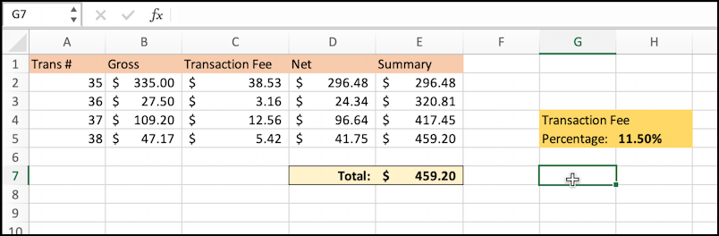
I have a demo spreadsheet on my computer for just this sort of task [download a copy]. It’s pretty rudimentary but do notice that the calculations are based on information spread across the sheet: “Transaction Fee” is calculated by Gross * Transaction Fee Percentage:

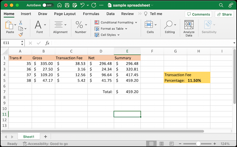
I’ve already done some basic formatting by adding background color fills to the spreadsheet, but let’s focus our attention on the “Total” cell (D7) and the calculated value (E7). To start, click on the cells to choose them, then choose “Font” from the ribbon bar along the top:

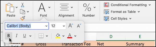
Here it’s showing me quite a few formatting options, including font, size, and more. To make the word “Total” and the calculated value both appear in bold, a click on the “B” does the job.

ADD A FILL COLOR TO INDIVIDUAL CELLS

But let’s add a background fill too. That’s done by clicking on the paint bucket with the yellow swatch below it. A color grid appears:

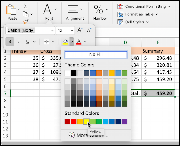
You can choose a theme color (did you know Excel supported “themes” to have your spreadsheets look more consistent? Learn more here: Excel Themes), or you can choose one of the standard colors. I’ll choose the bright yellow from that second palette.

But the cool kids actually choose something different from that Ribbon bar…

MICROSOFT EXCEL CELL FONT STYLES

In addition to the specific “Font” button, there are a couple of really useful shortcut links: Conditional formatting, Format as Table, and Cell Styles. Choose “Cell Styles” and lots of formats are shown:

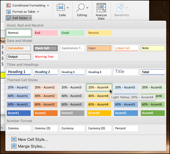
I always like the “Good, Bad and Neutral” cell formats, but there are a lot of options here that include borders, double borders, underlines, and much more. You can also choose a background fill by intensity. For example, I’m going to choose “20% – Accent 4” light yellow.

This is certainly the fastest way to get the results you want. But what if the combinations aren’t quite right or you want to apply more complex formatting, including specifying the type of data in the cell to ensure it’s shown correctly (like currency)?

DO IT YOURSELF CELL FORMATING IN EXCEL

The answer if you want to have maximal control over the formatting of a cell or group of cells you’ve selected is yet another button on the toolbar: “Cells“. Click on it and there are three options shown:

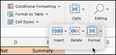
From here, choose “Format” and a submenu appears with quite a few choices and options:

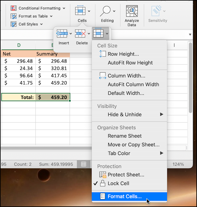
From a Mac user interface perspective, it’s interesting to have shortcut images appear on the menu; a very atypical user interface element. I like it, personally!

If what you want is on this menu, that’s great. If not, choose “Format Cells…” and you’ll be whisked into a completely different and quite complicated formatting window:

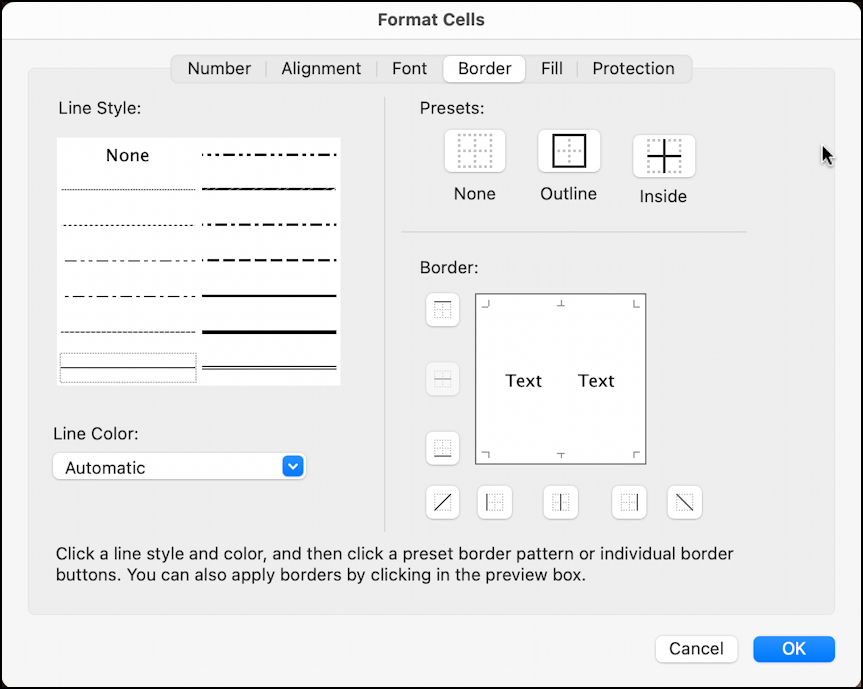
Notice along the top the categories: Number, Alignment, Font, Border, Fill, and Protection. Above you can see the “Border” option, and it really does give you oodles of options to set up the border exactly as you’d prefer.

I’m going to choose “Outline” and pick a heavier line from the style list on the left. The preview changes:

A click on “OK” and it’s applied…

A lot of different ways to format those two cells, but as you can see, there’s also a remarkable amount of power and flexibility hidden in Microsoft Excel. Ya just gotta explore and experiment. In fact, you can download my test spreadsheet if you want to experiment with it too. A good thing to do while stuck in a boring Zoom meeting. 🙂

Pro Tip: I’ve been using and writing about Microsoft’s Office Suite for many years. Please check out my Outlook help library for plenty of useful tutorials, as well as my additional Microsoft Office 365 help pages! Thanks.