How Do I Set Up A Basic Spreadsheet with Formulas in Microsoft Excel?

Spreadsheets have been around almost as long as we’ve had personal computers, starting with VisiCalc back in 1979. Yes, there were commercial computer programs released that long ago! Imagine, that’s forty-three years ago. What’s even more amazing is that the basic concepts haven’t changed much at all, with every ‘cell’ identified by a column/row pairing and formulas referencing those cells. Now we can do 3D transformations and pivots, but at their most basic, spreadsheets have remained extraordinarily similar for all of those forty-three years.

What you’re talking about is also a classic financial modeling task: how does changing this value affect the rest of the spreadsheet? That was its first really big task, actually, and what made spreadsheets so astonishingly useful compared to a paper ledger (that was used for hundreds of years in business and might be how you still reconcile your checking account). Excel was first released in 1985, but was originally MultiPlan, as released in 1982. Yes, that fancy Excel program you’re using has a long, storied history too.

But let’s jump into your task.

HOW TO FIGURE OUT RETAIL COST WITH A SPREADSHEET

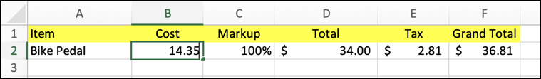
The most basic calculation for retail is that the shelf-price of a product is 2x the cost of the product. That’s 100% markup. Some retailers use a slightly different “keystone” formula where it’s actually a 110% markup, but the basic idea is the same. Tax is easily calculated as base cost + (base cost * tax rate), and the final price for a customer is shelf-price + tax. Here’s how I’d model that for a bike pedal:

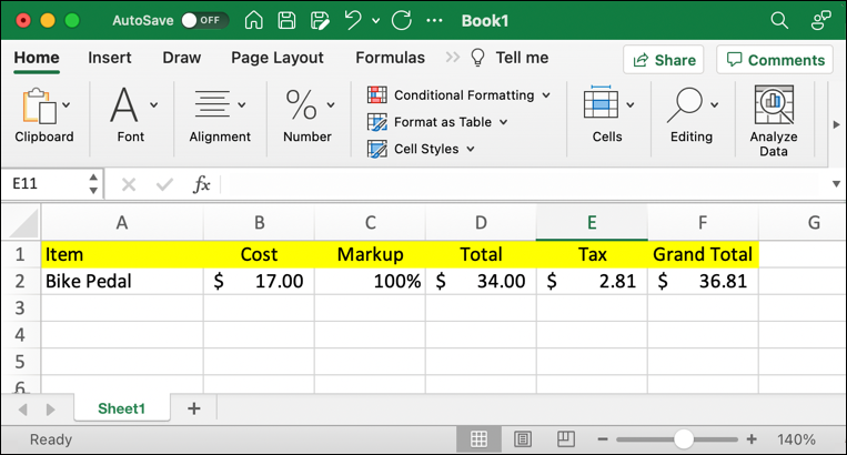
You can see that for a bike pedal that costs $17, the final price including tax is going to be $36.81. But how is this calculated?

To find a formula in a spreadsheet, simply click on the cell and press Return. In the case of

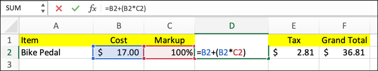
You can see that the cell D2 is actually a formula

=B2+(B2*C2)

So the product price is base price + (base price * markup). Essentially, 2x the price, but I’ve written it this way so that if we decide to have a 70% markup or a 113.5% markup, the spreadsheet will still work properly.

Notice that the formula both shows up in the cell and on the toolbar above it.

Now, how is tax being calculated? A click on E2 reveals the formula:

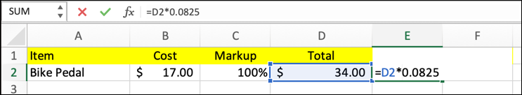
The tax rate is what’s known as hardcoded into the formula, which we’ll fix in a little bit, but for now you can see that the formula is

=D2*0.0825

That’s a tax rate of 8.25%, which is the tax rate we pay in my hometown of Boulder, Colorado.

Finally, the grand total price is total price + tax:

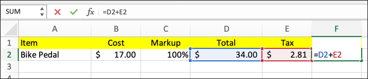
Simple enough this time: D2 + E2.

Notice when you’re viewing a formula that the referenced cells gain colored backgrounds that match the colors of their cell values. A handy shortcut if you’re trying to figure out why something isn’t working correctly.

MODELING PRICE CHANGES BASED ON COST CHANGES

The real value of this sort of spreadsheet, of course, is to answer questions like “what happens if…”. For example, what would happen if we switched to a different retailer and could acquire those bike pedals for a lower price?

I simply enter a different value in the Cost cell, as shown above, and once I press Return to have it accepted as the value, everything else immediately changes and updates based on the formula specified:

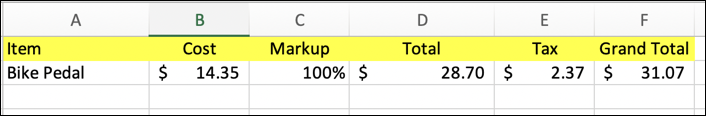
You can see that by dropping the wholesale cost from $17.00 to $14.35 (a difference of $2.65) the final price difference actually ends up being $5.74. Logical. But what happens if we move our business to a different location with a different tax rate? Well, let’s fix up this spreadsheet to better allow these type of tests…

HOW TO USE REFERENCE CELLS

I always like to have a small area on the side of my spreadsheets that clearly list all the assumptions and multiples. For taxes, we can do that thusly:

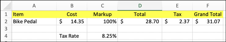
To get this to work, the formula calculating tax in E2 is updated to:

=D2*C4

Now if you wanted to change the tax rate from 8.25% (which is, of course, identical to 0.0825) it’s easy to do, even if there are a half-dozen or thousands of products in your spreadsheet.

Heck, while we’re at it, let’s make that markup a bit more obvious too:

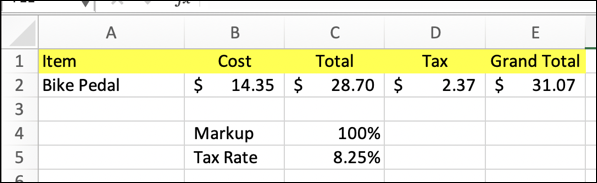
Now I can pull the “Markup” column out entirely (*since it’d be the same for every product anyway), making the overall spreadsheet much simpler. This change also means that modeling different retail pricing approaches – 80% markup? 115% markup? – become a breeze too.

There are a million directions you can go from here, but this will at least get you started. Next up you’ll want to read about Relative versus Absolute cell references, so as you duplicate that one inventory line, all the references work correctly. Start here: Relative vs Absolute Cell References In Excel. You can also pick up a lot of handy formatting tips in this tutorial: Get Started Formatting Your Excel Spreadsheet.

Pro Tip: I’ve been writing about computing basics and Microsoft Office since the early days. Heck, I remember VisiCalc on the Apple II. Please check out my extensive Microsoft Office 365 help area for lots and lots more useful tutorials while you’re visiting! Thanks.