How To Get Started Building an Excel Spreadsheet?

I don’t know if I’m supposed to keep this a secret so I don’t sound too nerdy, but I actually love working on spreadsheets. Both the formatting and the formula entry are fun and satisfying in much the same way that adding a piece to a jigsaw puzzle is fun. Watch an old movie and you’ll see people with their big ledgers, painstakingly entering lines of data and calculating the addition or subtraction of values to keep a running total. It’s painful. Ever since the introduction of VisiCalc back in 1979, digital spreadsheets have been one of the killer apps for computers overall. Now, of course, they’re quite a bit more sophisticated, but a checkbook ledger is quite straightforward: You subtract checks you write, and you add deposits you make.

The main thing to realize when you’re building a spreadsheet is that each box on the spreadsheet is a “cell” and that a cell can contain text, numbers, dates, unformatted text or a formula. The formula itself can then depend on and reference other cells in the spreadsheet, which is where it gets so interesting. This way you can have a fixed value for, say, starting balance, then have all credits and debits (a credit is an addition to the account, and a debit is a subtraction) relative to that value. Change your starting balance and that change bubbles through the entire ledger, for a few, a few dozen or even hundreds of entries. It can be darn cool!

BUILD A BASIC EXCEL SPREADSHEET

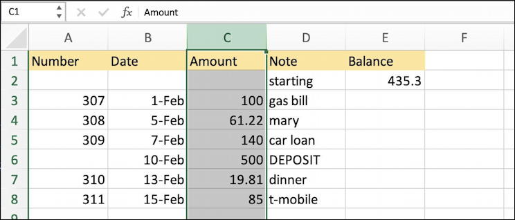
To start out, open up Microsoft Excel and enter some sample transactions for a checking ledger. Those are usually comprised of five fields: check number, date, amount, payee and a running balance. Without any formatting at all, here’s my basic checkbook ledger:

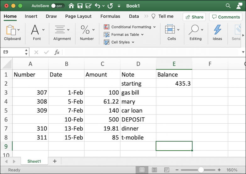
Notice that line 6 is a deposit of $500. And just in time; the balance is running rather low, as you’ll see once we flesh out this spreadsheet! Let’s start with changing some cell background colors to make it a bit easier to read. And so, our first trick: Any formatting you can apply to one cell you can do to a group of cells by selecting them all first. So click and drag to select all five column titles, from Number (cell A1) to Balance (cell E1).

Then choose Cells > Format > Format Cells… from the “ribbon” (the toolbar at the top of Excel. It’ll look like this:

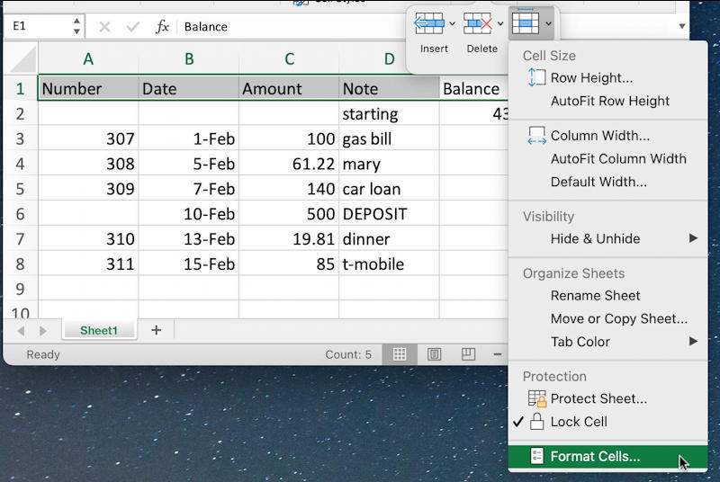
Once you’re in the format cells area, there’s quite a lot you can do. First off, you can specify the data format so that currency values are displayed properly, dates, and, well, check it out:

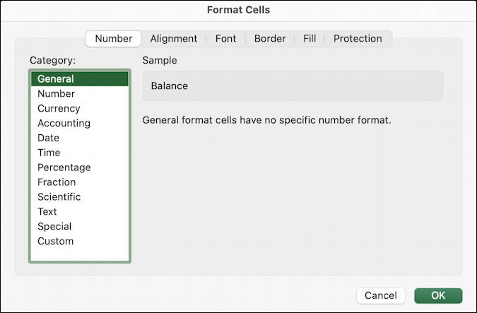
Excel does a really good job of explaining things, so you can click on the various format options and it’ll show examples. But for right now, click on “Fill” along the top. A color palette shows up with lots of cheery fill (background) colors:

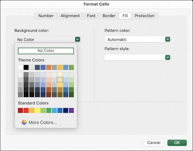
You can go wild here, but I’ll be relatively restrained by using a subtle yellow background for the column heads. Choose the color, then click “OK” to proceed and the spreadsheet already looks better!

Now click on the “C”: Turns out you can click on a column head to choose every cell in that column, or a row number to choose every cell in that row. Here’s column “C” selected:

Now instead of going through the clumsy menu system off the Ribbon instead right-click on one of the selected cells (on a Mac you’ll need to Control-click instead). A context menu pops up:

Aha! “Format Cells…” is easier to access here. Notice that there’s also a keyboard shortcut too. On the Mac it’s Command-1. Easy.

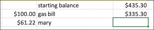
Choose “Currency” from the formatting options and then do the same for the Balance column (column “E”). Now things are looking good and it’s time to…

ENTER A FORMULA INTO AN EXCEL SPREADSHEET

To calculate the running balance of your checkbook ledger, you need to use the formula previous balance – amount of check. To enter it as a formula, click on the cell where the value should be displayed, then type the equals sign “=”.

You’ve now moved into formula entry mode and for basic formulas it’s surprisingly easy. Just click on the cell you want to reference and its “address” will appear in the formula cell. Enter any mathematical notation to express the relationship between cells, then click on the next cell value you want to reference. Here’s what I get:

To produce this formula, I typed in “=”, clicked on the starting balance cell (E2), typed “-“, then clicked on the amount of this particular check, cell C3. Press Enter or Return and the value is calculated and you’ve got your first formula in your spreadsheet!

Here’s what most people don’t realize with Excel: You can copy and paste formula and it will automatically tweak it to make sense in the current cell. For example, now that the formula in cell E3 is correct, click on the cell and choose Edit > Copy, then click on the cell you want to duplicate the formula (immediately below):

Now just microsoft excel basics – checkbook ledger – and you’ll see it actually changes the formula to =E3-C4 as you would desire!

Two things of note here: 1. You can always view a formula by clicking on the cell in question and 2. If you want to lock a specific cell reference location, add “$”. So if for some reason you wanted to have the second check be starting balance – check value regardless of where it is in the spreadsheet, use $E$2 instead of E2. That’s a general rule so you can use it even in quite complex formula!

Now you can just copy and paste the formula into each cell in the Balance column. Right? Wrong. What about that deposit?

One way you could address it is to always enter deposits as negative values, so a $500 deposit would be entered as -500, or, for that matter, deposits could be positive, but all check values are entered as negative numbers. Or you could just use a different formula for that one cell, where its value is the value of the cell above it PLUS the amount of the deposit:

Finally, here’s my check ledger spreadsheet:

To denote that deposit lines are different, I’m going to click and drag to select the cells in that row, then apply a light green fill to that set of cells. Easy to do, just like the yellow background fill for the column heads.

Where you can immediately see the value of this spreadsheet is when you realize that your starting balance was wrong. Instead of $435.30 it should have been $495.22. Since you have a spreadsheet based on actual formula calculations, changing that one cell at the top immediately changes every single value, offering a different final running balance as you would hope:

Easy once you get the hang of it, right?

There’s a lot more you can do to make your spreadsheets useful, including a lot of formatting options (I’d probably change those date formats to start, and center align the column heads) but this should be enough to get you started creating your own Excel spreadsheet. Remember, big, complex spreadsheets start out just as rudimentary in the beginning too.

Pro Tip: I’ve been writing about computing basics and Microsoft Office since the early days. Heck, I remember VisiCalc on the Apple II. Please check out my extensive Microsoft Office 365 help area for lots and lots more useful tutorials while you’re visiting! Thanks.